Electronic Supplement to
Resolution of non-double-couple-mechanisms: simulation of hypocenter mislocation and velocity structure mismodeling
by Jan Šílený
Shear-tensile source: α = 10°

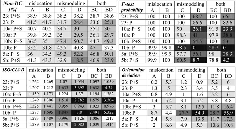
Station configurations from Fig. 3 are considered: 23, 10a, 10b, 5a, 5b. In the configurations 23, 10a, 10b two inversion options are considered: (i) P+S indicates that the inversion includes both P and S amplitude data, while (ii) P indicates that only P amplitudes are included in the inversion. In the configurations 5a and 5b the case (i) only is considered, as the case (ii) represents an underdetermined inverse problem. For each configuration, in turn, the inversions were performed using GF constructed for
(A) the hypocenter mislocated in depth,
(B) the hypocenter mislocated both in the depth and the horizontal coordinates,
(C) a simplified velocity model – layered 1-D model replaced by a homogeneous halfspace,
(D) even more simplified velocity model – the 1-D velocity model replaced by a homogeneous space,
(BC) combination of (B) and (C),
(BD) combination of (B) and (D).
For quantitative details about the cases (A-D) see the last paragraph of the section Set-up of the experiment. The four tables composing the Figure summarize the quantities characterizing the MT resolution:
- the percentage of non-DC components (top left), for the theoretical values see Tab. 1,
- the ratio of the ISO percentage and CLVD percentage ISO/CLVD (bottom left), the theoretical value being 5/4 for Lame’s constants λ=μ,
- the probability (in percents) that the MT model is significant, obtained in the F-test comparing the unconstrained MT and pure DC model, and
- the deviation (in degrees) of the orientation of the retrieved mechanism in the MT representation from the theoretical model used to synthesize the data, expressed as the sum of deviations for all 3 principal axes (bottom right).
Grades of shade mark qualitatively the size of the deviation of the quantities (1-4) from their theoretical values: the bigger deviation, the darker shade.